What is Pycaret

Pycaret is a new machine learning library that simplifies machine learning workflows. It is a high level library that sits on top of the most popular ML libraries - including general purpose libraries such as scikit-learn, tree-based such as lightgbm, xgboost and catboost, and NLP libraries such as nltk, gensim and spacy. In a sense pycaret shifts the focus from the implementation of mathematical algorithms to the implementation of ML workflow algorithms. Some of pycaret's functions, such as setup, create_model, predict_model, plot_model, are meant to perform a part of a typical data science project, while abstracting away from how the actual libraries underneath operate.

In this sense it is a little bit like build tools Maven and Gradle, tools that did not really care how the underlying tools in your project operated but focused instead on the workflow of producing build artifacts at the end. It is more of an ML workflow library with a set of opinionated workflow algorithms that guide how a data science project is created.

If you recall Maven artifacts are written in the scripting language most familiar to developers at the time - XML. Jupyter notebooks have the same familiarity for data scientists now - most data scientists use them. Pycaret is unapologetically intended for use in Jupyter notebooks - several of the functions output data to be displayed in a notebook as the data science project is being created. So for example, - when you load using get_data - it displays the data that was loaded in the notebook. This makes use of the IPython.display. Pycaret also uses ipywidgets to show tabs or other UI elements useful to assist a data scientist while working on a data science project. This is familiar to me - I have written a few Jupyter first libraries of my own

Getting Started

To get started install pycaret. In the best case scenario it's a simple as

pip install pycaret

For more details go to the Pycaret Install page

Included Datasets

Pycaret includes several datasets to get started with. To use the included data, import the datasets package from pycaret.

from pycaret.datasets import get_data

Included with pycaret is a small dataset called juice. This small dataset has information about 1070 purchases of Citrus Hill or Minute Maid orange juice. It is originally meant for R projects and so is hosted on rdrr.io, a site where searching for R related packages and data. Because the data is small, it is conveniently included in the pycaret library.

To get the data use the get_data function. This conveniently also displays the data in the notebook.

juice_dataset = get_data('juice')
Id Purchase WeekofPurchase StoreID PriceCH PriceMM DiscCH DiscMM SpecialCH SpecialMM LoyalCH SalePriceMM SalePriceCH PriceDiff Store7 PctDiscMM PctDiscCH ListPriceDiff STORE
0 1 CH 237 1 1.75 1.99 0.00 0.0 0 0 0.500000 1.99 1.75 0.24 No 0.000000 0.000000 0.24 1
1 2 CH 239 1 1.75 1.99 0.00 0.3 0 1 0.600000 1.69 1.75 -0.06 No 0.150754 0.000000 0.24 1
2 3 CH 245 1 1.86 2.09 0.17 0.0 0 0 0.680000 2.09 1.69 0.40 No 0.000000 0.091398 0.23 1
3 4 MM 227 1 1.69 1.69 0.00 0.0 0 0 0.400000 1.69 1.69 0.00 No 0.000000 0.000000 0.00 1
4 5 CH 228 7 1.69 1.69 0.00 0.0 0 0 0.956535 1.69 1.69 0.00 Yes 0.000000 0.000000 0.00 0

The data seems complete and mostly numeric. The only weird thing about the data is that Id column, which we do not need because pandas generates an index for us. So let's drop it.

if 'Id' in juice_dataset:
    juice_dataset = juice_dataset.set_index('Id')

Get Data Niceties

The get_data function has a couple of nice options. With save you can save a copy of the data in the local filesystem. With profile you can output a pandas profile report. You can see more details about get_data by running get_data?? in a code cell

Pandas Profiling Report

When you include the profile parameter get_data will output a pandas_profiling report created using the pandas_profile library. This gives a lot of information about the dataset and its features. Normally this helps in the data exploration phase of a data science project, but it's nice to also have it included in a function to get data.
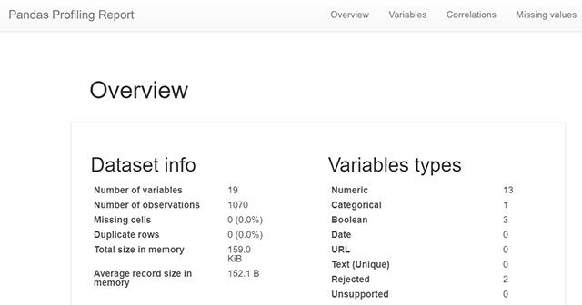
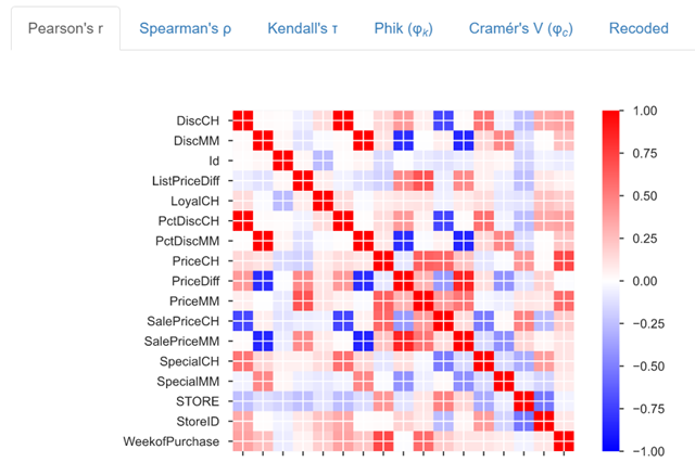
Pandas Profiling Report Pandas Profiling Report

More about the orange juice dataset

We can find out more about the juice dataset by visiting the webpage at rdrr.io. Aternatively, we can grab the html from the site and convert the data description into a pandas dataframe. For this we will use a requests and BeautifulSoup. Here is that code.

#collapse
import pandas as pd
from bs4 import BeautifulSoup
import requests

pd.options.display.max_colwidth = 120

# 1. Grab the HTML from the website
r = requests.get('https://rdrr.io/cran/ISLR/man/OJ.html')

# 2. And convert it to a BeautifulSoup object
soup = BeautifulSoup(r.text)

def find_cells(soup, element):
    for dl in soup.find_all('dl'):
        for dt in dl.find_all('dt'):
            
            # 3. Once we find the <dt> element return it along with the <dd> element
            yield dt.text.strip(), dt.nextSibling.text.strip().replace('\n', ' ')
            
# 4. Convert the generator to a list of tuples
dt = list(find_cells(soup, 'dt'))

# 5. Now create a dataframe from the list of tuples
pd.DataFrame(dt, columns=['Feature','Description']).style.hide_index()

Feature Description
Purchase A factor with levels CH and MM indicating whether the customer purchased Citrus Hill or Minute Maid Orange Juice
WeekofPurchase Week of purchase
StoreID Store ID
PriceCH Price charged for CH
PriceMM Price charged for MM
DiscCH Discount offered for CH
DiscMM Discount offered for MM
SpecialCH Indicator of special on CH
SpecialMM Indicator of special on MM
LoyalCH Customer brand loyalty for CH
SalePriceMM Sale price for MM
SalePriceCH Sale price for CH
PriceDiff Sale price of MM less sale price of CH
Store7 A factor with levels No and Yes indicating whether the sale is at Store 7
PctDiscMM Percentage discount for MM
PctDiscCH Percentage discount for CH
ListPriceDiff List price of MM less list price of CH
STORE Which of 5 possible stores the sale occured at

Preparing Data

First, we split the data into training and test set. It is a small dataset and maybe we can get by with an 80/20 split, especially since we will use tree based algorithms or similar algorithms that can handle small datasets.

train = juice_dataset.sample(frac=0.80)
unseen_data = juice_dataset.drop(train.index).reset_index(drop=True)

train.shape, test.shape
((856, 18), (214, 18))

The setup function

At the heart of Pycaret has a powerful machine learning pipeline that takes the input data and performs a huge part of the traditional data processing workflow. This pipeline is started by calling the setup function. setup initializes the environment, and creates the data transformation pipeline to prepare the data for model training.

It is a bit of a magic function - a lot of work is done inside this function and it has to be called before any of the pycaret model development is started. You call setup on your training data and tell it the target variable, and it will start preparing for model training. Importantly, it does some of the work that data scientists would be doing manually at this point, including making decisions about some of the preprocessing steps, such as apply PCA, or removing outliers etc. How well it does this is yet to be seen but it is certainly a big change to a data scientist's workflow if this can be done automatically. A lt of steps are done automatically by pycaret, as we will see later.

Regardless, setup displays a dataframe with information it discovers about the data's features and includes some of the decisions that were taken. This give a nice platform for ML modeling.

from pycaret.classification import *

juice_prep = setup(train, target='Purchase')
 
Setup Succesfully Completed!
Description Value
0 session_id 2574
1 Target Type Binary
2 Label Encoded CH: 0, MM: 1
3 Original Data (856, 18)
4 Missing Values False
5 Numeric Features 12
6 Categorical Features 5
7 Ordinal Features False
8 High Cardinality Features False
9 High Cardinality Method None
10 Sampled Data (856, 18)
11 Transformed Train Set (599, 16)
12 Transformed Test Set (257, 16)
13 Numeric Imputer mean
14 Categorical Imputer constant
15 Normalize False
16 Normalize Method None
17 Transformation False
18 Transformation Method None
19 PCA False
20 PCA Method None
21 PCA Components None
22 Ignore Low Variance False
23 Combine Rare Levels False
24 Rare Level Threshold None
25 Numeric Binning False
26 Remove Outliers False
27 Outliers Threshold None
28 Remove Multicollinearity False
29 Multicollinearity Threshold None
30 Clustering False
31 Clustering Iteration None
32 Polynomial Features False
33 Polynomial Degree None
34 Trignometry Features False
35 Polynomial Threshold None
36 Group Features False
37 Feature Selection False
38 Features Selection Threshold None
39 Feature Interaction False
40 Feature Ratio False
41 Interaction Threshold None

Compare Models

Once the data is prepared, a data scientist would now choose among candidate models. Again, there is another magic function compare_models which does this for you. This runs several models - 15 as shown below - on the data , and display key metrics to allow ypu to choose among the model types for the next step.

compare_models()
Model Accuracy AUC Recall Prec. F1 Kappa
0 Extreme Gradient Boosting 0.826500 0.893900 0.771300 0.792000 0.779900 0.636900
1 Linear Discriminant Analysis 0.824800 0.904300 0.776000 0.785100 0.780100 0.634500
2 Logistic Regression 0.823100 0.901500 0.746800 0.801700 0.771100 0.627400
3 Ridge Classifier 0.819800 0.000000 0.767700 0.780500 0.773300 0.623700
4 Ada Boost Classifier 0.816500 0.884300 0.738300 0.795000 0.762900 0.613700
5 Gradient Boosting Classifier 0.816500 0.893800 0.758800 0.780100 0.767000 0.615800
6 Random Forest Classifier 0.803100 0.869800 0.705200 0.787600 0.741200 0.583200
7 CatBoost Classifier 0.803100 0.892100 0.742200 0.762700 0.747500 0.586800
8 Light Gradient Boosting Machine 0.796400 0.886400 0.721200 0.762500 0.737000 0.571600
9 Extra Trees Classifier 0.771300 0.846400 0.696700 0.726200 0.707900 0.520500
10 Naive Bayes 0.769700 0.837100 0.775800 0.690400 0.729000 0.530000
11 Decision Tree Classifier 0.769600 0.759200 0.696700 0.721200 0.706100 0.517100
12 K Neighbors Classifier 0.702700 0.740700 0.563500 0.653100 0.600400 0.366900
13 Quadratic Discriminant Analysis 0.656200 0.699000 0.599200 0.594300 0.565100 0.292900
14 SVM - Linear Kernel 0.535700 0.000000 0.616700 0.375700 0.420200 0.104500

Available Models

pd.read_csv('pycaret_models.csv').style.hide_index()
Estimator Abbreviated String Original Implementation
Logistic Regression lr linear_model.LogisticRegression
K Nearest Neighbour knn neighbors.KNeighborsClassifier
Naives Bayes nb naive_bayes.GaussianNB
Decision Tree dt tree.DecisionTreeClassifier
SVM (Linear) svm linear_model.SGDClassifier
SVM (RBF) rbfsvm svm.SVC
Gaussian Process gpc gaussian_process.GPC
Multi Level Perceptron mlp neural_network.MLPClassifier
Ridge Classifier ridge linear_model.RidgeClassifier
Random Forest rf ensemble.RandomForestClassifier
Quadratic Disc. Analysis qda discriminant_analysis.QDA
AdaBoost ada ensemble.AdaBoostClassifier
Gradient Boosting gbc ensemble.GradientBoostingClassifier
Linear Disc. Analysis lda discriminant_analysis.LDA
Extra Trees Classifier et ensemble.ExtraTreesClassifier
Extreme Gradient Boosting xgboost xgboost.readthedocs.io
Light Gradient Boosting lightgbm github.com/microsoft/LightGBM
CatBoost Classifier catboost https://catboost.ai

Create Model

Assuming we decide to use the Ridge Classifier, then the next function is intuitively create_model. This will create a Ridge Classifier model with default hyper parameters.

rc = create_model('ridge')
Accuracy AUC Recall Prec. F1 Kappa
0 0.8000 0.0 0.7500 0.7500 0.7500 0.5833
1 0.8000 0.0 0.7500 0.7500 0.7500 0.5833
2 0.8667 0.0 0.8333 0.8333 0.8333 0.7222
3 0.7833 0.0 0.6667 0.7619 0.7111 0.5390
4 0.8500 0.0 0.8333 0.8000 0.8163 0.6897
5 0.8167 0.0 0.7083 0.8095 0.7556 0.6099
6 0.8833 0.0 0.8750 0.8400 0.8571 0.7586
7 0.7500 0.0 0.6667 0.6957 0.6809 0.4755
8 0.7833 0.0 0.7600 0.7308 0.7451 0.5568
9 0.8644 0.0 0.8333 0.8333 0.8333 0.7190
Mean 0.8198 0.0 0.7677 0.7805 0.7733 0.6237
SD 0.0418 0.0 0.0700 0.0471 0.0554 0.0885

Tune Model

Instead of create_model, which uses default parameters and so might not have optimal performance, you can call tune_model. This will automatically tune the model's hyperparameters.

ridge_tuned = tune_model('ridge')
Accuracy AUC Recall Prec. F1 Kappa
0 0.8000 0.0 0.7500 0.7500 0.7500 0.5833
1 0.8000 0.0 0.7500 0.7500 0.7500 0.5833
2 0.8833 0.0 0.8750 0.8400 0.8571 0.7586
3 0.7833 0.0 0.6667 0.7619 0.7111 0.5390
4 0.8500 0.0 0.8333 0.8000 0.8163 0.6897
5 0.8167 0.0 0.7083 0.8095 0.7556 0.6099
6 0.8833 0.0 0.8750 0.8400 0.8571 0.7586
7 0.7500 0.0 0.6667 0.6957 0.6809 0.4755
8 0.7833 0.0 0.7600 0.7308 0.7451 0.5568
9 0.8644 0.0 0.8333 0.8333 0.8333 0.7190
Mean 0.8214 0.0 0.7718 0.7811 0.7757 0.6274
SD 0.0439 0.0 0.0749 0.0479 0.0584 0.0931

Plot Model

Another nice feature that pycaret provides is the ability to plot different charts that can tell you how your model performs. For our ridge classifier we can plot a Precision-Recall Curve using plot_model(plot='pr'). There are many different types of plots and it would be cool to try them out.

plot_model(ridge_tuned, plot = 'pr')

Predict

Finally, when we call predict_model pycaret runs the predictions and appends the labels to the original data.

unseen_predictions = predict_model(ridge_tuned, data=unseen_data)
unseen_predictions[['Purchase', 'Label']]
Purchase Label
0 MM 1
1 CH 0
2 CH 0
3 MM 1
4 CH 0
... ... ...
209 CH 0
210 MM 1
211 CH 0
212 MM 1
213 MM 0

214 rows × 2 columns

Conclusion

pycaret is fun to use and it is useful.